Nonlinear Dynamical Systems - Van der Pol Oscillator

Background

Back when I was in school, I took a course on nonlinear differential equations and chaotic dynamical systems, and man was that class fun. The instructor emphasized using qualitative techniques pioneered by the likes of Poincaré and others at the turn of the last century to obtain information about the global behavior of complicated dynamical systems, as opposed to using intensive numerical methods to attempt to find valid analytical extensions for certain solutions. Personally, I found the qualitative technique a lot more satisfying, since it appealed to the monkey part of my brain that needs pictures to help me gain insight into literally anything.

A differential equation (diff eq) is an equation that relates one or more unknown functions and their derivatives, and they have been central in the study of math and physics since antiquity. When applied to specific physical problems, these functions generally represent physical quantities, the derivatives represent rates of change for the aforementioned quantities, and the differential equation defines a relationship between the two. As the study of differential equations gained in interest and notoriety, it became increasingly clear to all who dabbled in the material that there were inherent limitations to even the most reliable numerical methods. Problems had gotten too complicated, and our ability to find or prove closed form solutions to problems paled in comparison to the steady volume of interesting problems to consider.

Poincaré shifted the paradigm, abandoning the need for numerical or approximate solutions. Instead, he and his contemporaries focused on understanding how local dynamics near extrema sets contributed to the larger-scale qualitative picture that the global phase portrait of a system depicts. These advances gave us robust tricks to understand even the dynamics of nonlinear systems, which are notoriously more difficult to analyze when compared to their linear counterparts.

Technical Jargon

For our investigations, we will be generally concerned with diff eqs of the form \(\dot{x} = f(x,t)\), meaning we can describe the motion of \(x\) through \(t\) as a function \(f(x(t))\). I’m not prepared to give a full crash course in dynamical systems theory here today, but for completeness sake I’ll provide the formal definition for a handful of key objects in our toolbox. Hopefully this imparts some intuition to the reader about how to use these objects

Differential Eqs & Dynamical Systems

Okay, lets get the core definitions out of the way first!

Definition: Differential Equation

Quite simply, a differential equation is just an equation that expresses the derivative of an independent variable (lets say \(x\)) with respect to a dependent variable (lets say \(y\)). Or in formal notation, a differential equation expresses:

\[\frac{dy}{dx} = f(x)\]

In our case, we will consider position in the space (dependent) to be a function of time (independent). So really,

\[\frac{dx}{dt} = \dot{x} = f(x)\]

Definition: Dynamical System

a (one parameter) dynamical system on \(E\) is a \(C^1\)-map

\[\psi: \mathbb{R} \times E \to E\]

where \(E \subset \mathbb{R}^n\) is open and if \(\psi_t(x) = \psi(t,x)\), then \(\psi_t\) satisfies

• \(\psi_0(x) = x\), \(\forall x \in E\)
• \(\psi_t \circ \psi_s(x) = \psi_t (\psi_s(x))\)= \(\psi_{t+s}(x)\)

For each \(t \in \mathbb{R}\), \(\psi_t\) maps \(E\) into \(E\) continuously, with a continuous inverse \(\psi_{-t}\). In other words, \(\psi_t\) is a one parameter family of diffeomorphisms on E, forming a commutative group under function composition.

Intuitively, this object describes a family of solution curves to a diff eq in \(\mathbb{R}^n\). If we think of the diff eq as describing the motion of a fluid, then each single curve describes the trajectory of an individual particle in the fluid. The flow of the dynamical system describes the motion of the entire fluid.

Def: Phase Portrait

A phase portrait shows the set of all solution curves to the diff eq. Geometrically, this depicts an \(n\)-dimensional space populated by the trajectories to solutions of the diff eq, where \(n\) corresponds to dimension of the system. Its usually most convenient to restrict our view to a phase plane, which is a fancy name for the 2-d phase portrait.

Aside: Notation

I’ve often seen authors use \(\dot{x}\) to depict the time derivative of the spacial function \(x(t)\), as opposed to writing out \(\frac{dx}{dt}\), and I will be no exception. I just wanted to mention this explicitly in case anyone is following at home, and wondered what all the dots were about.

Analysis: Van Der Pol Oscillator

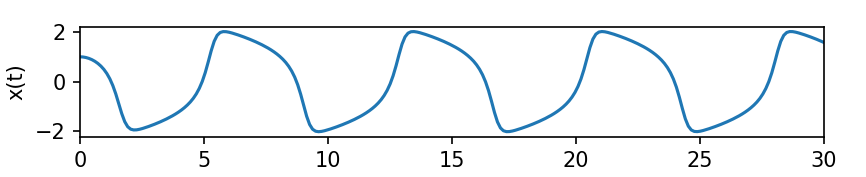
Today I want to present a brief analysis of the dynamics of the simple homogeneous Van Der Pol (VDP) oscillator. Figure 1 characterizes the dynamics of this oscillator through time.

\[{d^2x \over dt^2} - r(1-x^2) {dx \over dt} + x = 0 \tag{1}\]

Note that this is an autonomous second order differential equation in the position coordinate \(x\), which as we mentioned, is really a function depending on the time parameter \(t\). The scalar \(r\) characterizes the “strength” of the nonlinear dampening, and is usually thought to be nonnegative (\(0 \leq r\)). In our case, autonomous means that even though \(x\) should really be thought of as \(x(t)\), a function of the time parameter \(t\), the system’s overall behavior is characterized only by the evolution of \(x(t)\) and not \(t\) directly. Hence, it is time invariant, or autonomous, and we drop writing the explicit \(t\) to reduce visual clutter.

Also, note that we can present the evolution of trajectories for this system in a 2-dimensional phase space, so we should really think of \(x\) as tracking 2 spacial coordinates (i.e. \(x(t) = (x_1(t), x_2(t))\)). For the sake of brevity, I’ll drop referring to specific indexes unless required. To be explicit, if we set \(x_2 = \dot{x}\), we may transform the equation from figure 1 to the equivalent 2-d system described in figure 2.

\[\begin{equation}\begin{aligned} \dot{x_1} &= x_2 \\ \dot{x_2} &= r(1-x_1^2)x_2 - x_1 \end{aligned}\end{equation} \tag{2}\]

Before proceeding, consider the question of “what would motivate someone to study the dynamics of this equation?”, which is super fair. Its practical utility shines in providing a model for a nonlinear “relaxation-oscillator”. The Dutch electrical engineer Balthasar van der Pol , namesake for the equation in question, was one of the first to explore the applications of this diff eq to modeling the behavior of electrical circuits with vacuum tubes waaay back in the 1920’s and 30’s.

Relaxation oscillators are abundant in our modern world thanks to the ubiquity of electronics in our daily lives. Really the question isn’t “Why study this?”, but rather “Why wouldn’t you study this?”. Especially if your work deals with strange and silly oscillators on a daily basis.

Oh look, there goes one now!

Critical Point(s)

Recall that for a dynamical system, the critical (fixed) points are precisely the points where \(\dot{x} = {dx \over dt} = 0\). That is, the points where the rate of change of the position coordinate \(x\) with respect to the time parameter \(t\) is zero. Physically speaking, these are the points where the system is at a “steady state”, and is no longer moving. Or never was moving to begin with! In fact, one can show that no trajectory for a dynamical system that didn’t start or pass through a fixed point can reach a fixed point in finite time.

For our VDP Oscillator, by setting \(\dot{x} = 0\) we have the following:

\[\begin{equation}\begin{aligned} \ 0 &= x_2 \\ \ 0 &= r(1-x_1^2)x_2 - x_1 = -x_1 \end{aligned}\end{equation}\]

Algebraically, \(x_1 = x_2 = 0\) is the only point that satisfies these relations, so \((0,0)\) is the sole critical point for the VDP Oscillator. However, we still need to check the asymptotic stability of this point. In other words, we don’t know whether this point is attracting nearby orbits as \(t \to \infty\) , and is a stable equilibrium, or is repelling nearby orbits as \(t \to \infty\) an unstable equilibrium. Lets proceed to naively linearize about this fixed point to see if we can determine anything about the asymptotic stability of the system.

Recall linearizing means that for a specific fixed point \((\hat{x_1},\hat{x_2})\) of a dynamical system

\[\begin{align} \dot{x_1} &= f_1(x_1,x_2) \\ \dot{x_2} &= f_2(x_1,x_2) \end{align}\]

we find the closest linear approximation to the behavior of the system near this point by setting:

\[\begin{align} y_1 &= x_1 - \hat{x_1} \\ y_2 &= x_2 - \hat{x_2} \end{align}\]

To do this, we can expand these expressions out as a Taylor series in terms of the variables (\(y_1, y_2\)), discard any quadratic terms of \(y\) (aka \(O(y^2)\) where \(O(n)\) is of Big-O notation) and substitute \((\hat{x_1},\hat{x_2})\) where appropriate. More compactly, we can just look at the Jacobian (matrix of partial derivatives) for the original system:

\[\begin{align} f_1(x) &= x_2 \\ f_2(x) &= r(1-x_1^2)x_2 - x_1 \end{align}\] \[J = \begin{bmatrix} {\partial f_1 \over \partial x_1} & {\partial f_1 \over \partial x_2} \\ {\partial f_2 \over \partial x_1} & {\partial f_2 \over \partial x_2} \\ \end{bmatrix} = \begin{bmatrix} 0 & 1 \\ -2rx_1x_2-1 & r(1-x_1^2) \\ \end{bmatrix}\]

Evaluating the Jacobian at the critical point \((0,0)\) allows us to see that the linearization of the system has a Jacobian of

\[J_{(0,0)} = \begin{bmatrix} 0 & 1 \\ -1 & r \\ \end{bmatrix}\]

or, to be more explicit with our notation, the linearization about \((0,0)\) is:

\[\begin{bmatrix} \dot{x_1} \\ \dot{x_2} \end{bmatrix} = \begin{bmatrix} 0 & 1 \\ -1 & r \\ \end{bmatrix} \begin{bmatrix} x_1 \\ x_2 \end{bmatrix}\]

According to the Hartman-Grobman theorem, this linearized system should approximate the dynamics of the original system when we are close to the fixed point if it is hyperbolic. That is, provided that the eigenvalues of \(J\) are nonzero or have a nonzero real part (in the case of a complex eigenvalue). We can verify these criterion directly. First, we compute the characteristic polynomial for \(J\).

\[det(J- \lambda I) = \begin{vmatrix} -\lambda & 1 \\ -1 & r- \lambda \end{vmatrix} = \lambda^2 - r \lambda + 1\]

Then by the quadratic formula, we have eigenvalues \(\lambda_1 , \lambda_2\) such that

\[\begin{align} \lambda_1 =& {r + \sqrt{r^2 - 4}}\over{2} \\ \lambda_2 =& {r - \sqrt{r^2 - 4}}\over{2} \end{align}\]

Hmmm, it seems we’ve hit a bit of a snag here. The eigenvalues of this matrix are actually dependent on the value of \(r\), so we need to consider cases of \(r\) to complete our understanding of the dynamics about this fixed point. Typically, one only considers the cases where \(r \geq 0\), since this domain restriction more properly mimics original physical problem of dampening an oscillator. After all, how can you add negative friction to a physical system? For now, all we can say definitively describe are the following:

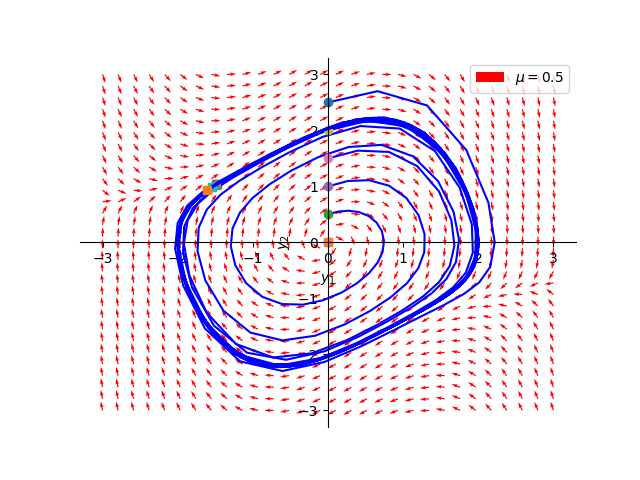
Subcase 1: \(0 \lt r \lt 2\)

Since the real parts of the eigenvalues for the linearized system are positive, the origin is unstable - so nearby trajectories are spiraling out from the origin as \(t \to \infty\). The origin \((0,0)\) is an unstable focus, due to the complex parts of the eigenvalues being nonzero. The figure below provides a view of the \(x_1,x_2\) phase portrait where \(r = 0.5\), including a handful of plotted trajectories.

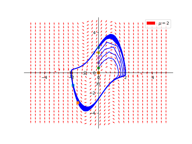
Subcase 2: \(r = 2\)

Here, we have a single eigenvalue \(\lambda = 1\) of multiplicity 2. The origin \((0,0)\) is therefore an unstable degenerate node, as depicted below.

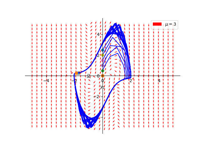
Subcase 3: \(r \gt 2\)

In this instance, both eigenvalues are now strictly positive and real, meaning the origin \((0,0)\) is an unstable node. Again, we show the phase portrait for an example of this case for completeness sake.

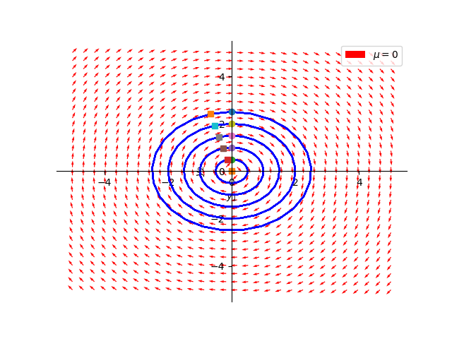
Subcase 4: \(r = 0\)

Since the real parts of the eigenvalues for the linearized system are zero, these eigenvalues are purely imaginary. In this case, the origin \((0,0)\) is a center. For a formal justification of why this is a center, continue to the next section. Here, solution curves are closed periodic trajectories that circle about the origin.

Limit Cycles & Liénard’s Theorem

When considering the behavior of a 2-dimensional dynamical system, there exists the possibility of a trajectory intersecting itself at a previous time, leading to certain trajectories having cyclic solutions. Just like fixed points, we can think about these periodic solutions as having attracting or repelling properties that influence the dynamics of a nearby trajectory’s asymptotic behavior.

A limit cycle, also called \(\omega\)-limit set, is a closed trajectory in phase space having the property that at least one other trajectory spirals into it either as time approaches infinity or as time approaches negative infinity. Physically, this expresses that there exists a periodic solution to the diff eq. Since we are modeling an oscillating system, it makes sense for us to consider the existence of limit cycles for the VDP equation. In fact, once we take care of this case, we’re almost done! Some heavy machinery from Poincaré and Bendixson assures us that fixed points and limit cycles are the only possible asymptotic behaviors that 2-d systems can exhibit.

Poincaré-Bendixson Theorem

Given a differentiable real dynamical system defined on an open subset of the plane, every non-empty compact \(\omega\)-limit set of an orbit, which contains only finitely many fixed points, is either:

• a fixed point,
• a periodic orbit,
• a connected set composed of a finite number of fixed points together with homoclinic and heteroclinic orbits connecting these.

This theorem also implicitly expresses that chaotic behavior is impossible for a 2-d dynamical system…. usually. There are some strange behaviors that arise when you consider the discrete version of certain continuous dynamical systems in \(\mathbb{R}^2\), but those are outside the scope of our current discussion. For now, lets return to an earlier case, where the dampening parameter \(r=0\).

Aside: Comparison to Simple Harmonic Oscillator

Recall the equation for the simple harmonic oscillator, probably the simplest 2nd order differential equation:

\[{d^2x \over dt^2} + x = 0\]

This has a known general solution of \(a \cos(t + \phi)\) where \(a, \phi\) are thought of as fixed constants. Note that this solution is periodic in \(t\). For our original equation for the VDP oscillator, if \(r = 0\) then the system reduces to

\[{d^2x \over dt^2} - (0)(1-x^2) {dx \over dt} + x = 0 \implies {d^2x \over dt^2} + x = 0\]

So the simple harmonic oscillator is a special case of the VDP oscillator! This fact is slightly underwhelming, but still important to recognize if we want to be thorough in our analysis. if we compute the eigenvalues of the Jacobian now, we see that they are purely imaginary (have zero real part).

\[\begin{align} \lambda_1 =& {0 + \sqrt{0^2 - 4}}\over{2} &= i\\ \lambda_2 =& {0 - \sqrt{0^2 - 4}}\over{2} &=-i \end{align}\]

Since these eigenvalues are purely complex, we can’t use Hartman-Grobman to justify the stability arguments we used for the linearization about \((0,0)\) in the case that \(r=0\). In other words, we can’t be sure that the linearized version of the system is actually equivalent to its nonlinear cousin in the case of a purely complex eigenvalue. We prematurely concluded that \((0,0)\) is a center in the previous section, but now we will invoke a symmetry argument thanks to a theorem from Perko’s book to justify our assertion.

Our system described in (2) actually permits the following symmetry. If we send \((x_1, x_2)\) to \((-x_1, -x_2)\), we claim that (2) is actually invariant with respect to this transformation. To see this, consider

\[\begin{equation}\begin{aligned} -\dot{x_1} &= -x_2 \\ -\dot{x_2} &= x_1-r(1-x_1^2)x_2 \end{aligned}\end{equation}\]

Which is exactly the same system as (2), so the VDP oscillator is symmetric with respect to both the \(x_1\) and \(x_2\) axis. Now, we invoke the aforementioned theorem

Theorem 2.10.6 (Perko)

Let \(E \subset \mathbb{R}^2\) be open containing the origin and let \(f \in C^1(E)\) with \(f(0) = 0\). If the nonlinear system is symmetric w.r.t the \(x_1\)-axis or \(x_2\)-axis, and if the origin is a center for the linearized system, then the origin is a center for the nonlinear system.

Boom! Based on the symmetry argument illustrated above and this theorem, we can safely conclude that at \(r=0\), the VDP oscillator is in fact a center.

As for the limit cycle, don’t panic just yet. We have some additional heavy machinery we can deploy to assist us.

Liénard’s Theorem

Consider the second order differentiable equation:

\[{d^2x \over dt^2} + f(x) {dx \over dt} + g(x) = 0 \tag{3}\]

Where the two functions \(f(x)\) and \(g(x)\) are continuously differentiable, \(f,g: \mathbb{R} \to \mathbb{R}\), with \(g\) an odd function and \(f\) an even function. This equation is commonly known as a Liénard Equation, and is a generalization of the dynamics of systems like the VDP equation.

Define the odd function \(F(x) := \int_0^x{f(s)ds}\). Due to a theorem from Liénard, we are guaranteed a unique, stable limit cycle surrounding the origin if the following conditions are met:

• \(\space g(x) > 0 , \space \forall x>\)0
• \(\space F(x)\) has exactly one positive root at some value \(p\), where \(F(x) < 0\) for \(0 < x < p\) and \(F(x) > 0\) and monotonic for \(x > p\)
• \(\lim\limits_{x \to \infty} F(x) := \lim\limits_{x \to \infty}{ \int_0^x{f(s)ds}} = \infty\) .

Applying Liénard’s Theorem

Consider the equation for the VDP equation (1), with \(f(x) = -r(1-x^2)\) and \(g(x) = x\). Recall that for our purposes, \(r \geq 0\). Clearly, \(g(x)\) is positive for positive \(x\). Also,

\[\begin{align} F(x) &= \int_0^x{f(s)ds} = \int_0^x{-r(1-s^2)ds} = r\int_0^x{(s^2-1)ds}\\ &= r(\frac{x^3}{3} - x) \end{align}\]

This cubic polynomial factors into

\[F(x) = rx(x^2-3) = rx(x - \sqrt{3})(x+\sqrt{3})\]

which has a single positive root \(p = \sqrt{3}\). Also, clearly \(\lim\limits_{x \to \infty} F(x) = \infty\). Now for the last conditions we proceed with reasoning by cases,

• if \(0 < x < \sqrt{3}\), then two factors of \(F(x)\) are positive but the \((x - \sqrt{3})\) factor would be negative. Thus \(F(x) < 0\)
• if \(\sqrt{3} < x\), then all three factors of \(F(x)\) are positive, so \(F(x)\) > 0. Moreover, \(F(x)\) will no longer change sign so it is monotonically increasing.

Since we’ve met all the conditions, we’ve confirmed that the VDP oscillator has a stable limit cycle about the origin!

Brief Numerical Methods

Having taken care of the broader qualitative analysis of the dynamics of the VDP oscillator, lets consider another approach. Namely, trying to determine a reliable approximation for the solution to this system using a bit of perturbation theory. Here, I’m going to refer to the dampening parameter \(r\) from before as \(\epsilon\) instead, to better reflect its nature as a slight perturbation parameter \(0 \leq \epsilon \lt 1\). Recall the normal form of the VDP oscillator and its general solution when \(\epsilon = 0\).

\[\ddot{x} - \epsilon (1-x^2)\dot{x} + x = 0 \space, \space a\cos(t+\phi)\]

where \(a \in \mathbb{R}\) and \(\phi \in [0, 2\pi)\) are constants. The idea is to see if we can recover a relatively faithful approximate solution to the original system near the critical point \((0,0)\) for small values of \(\epsilon\) by expanding the solution in powers of \(\epsilon\). In other words, our approximation will look something like a countably infinite polynomial in \(\epsilon\) with coefficients determined by the functions:

\[u(t;\epsilon) = u_0(t) + u_1(t)\epsilon + u_2(t)\epsilon^2 ...\]

where each \(u_n\) is a function dependent only on \(t\) and not \(\epsilon\), and \(u_0(t)\) corresponds to the solution of the base cause when \(\epsilon = 0\). We will attempt to substitute this expansion into the original differential equation and collect like coefficients for powers of \(\epsilon\). Note that since powers of \(\epsilon\) are linearly independent (a basic fact from linear algebra) the corresponding coefficients \(u_n\) must vanish independently if we want this expansion to hold for all values of small \(\epsilon\). So our strategy is to expand, collect coefficients, then try to solve the usually simpler \(u_n\) to find our approximation.

Aside: Asymptotics

Often when performing these expansions, we care more about the terms that “contribute” the most to the overall approximation than we do higher powers of \(\epsilon\). Since \(\epsilon\) is so small, we can safely assume that higher order parameters have a smaller magnitude than the lower order ones. This is all to say that when doing the algebra for these problems, I will often drop or ignore terms that are of \(O(\epsilon^3)\) or greater power. Its a bit sloppy, but we aren’t trying for perfect here, and for my purposes \(O(\epsilon^2)\) is a good enough approximation. However, our approximation is a bit naive, and will eventually “break down” as we get farther from the critical point \((0,0)\).

Lets begin by pulling the \(\dot{u}\) term to one side of the equals before substituting the expansion into the system and performing some algebraic manipulations. \(\begin{align} \ddot{u} + u &= \epsilon (1-u^2)\dot{u} \\ \ddot{u_0} + u_0 + (\ddot{u_1} + u_1)\epsilon + (\ddot{u_2} + u_2)\epsilon^2 + ... &= \epsilon(1-u_0^2 - u_0u_1\epsilon - u_0u_2\epsilon^2 - u_0u_1\epsilon - u_1^2\epsilon^2 - u_0u_2\epsilon^2 - ....) \\ & (\dot{u_0} + \dot{u_1}\epsilon + \dot{u_2}\epsilon^2 + ...) \\ &= (1-u_0^2)\dot{u_0}\epsilon - [(1-u_0^2)\dot{u_1} - 2u_0u_1\dot{u_1}]\epsilon^2 + O(\epsilon^3) \end{align}\)

Then based on our earlier observations about \(u_n\) and small \(\epsilon\), we can equate coefficients for like powers of \(\epsilon\)

• \(\epsilon^0\) : \(\ddot{u_0} + u_0 = 0 \implies u_0(t) = a\cos(t+\phi)\)
• \(\epsilon^1\) : \(\ddot{u_1} + u_1 = (1-u_0^2)\dot{u_0}\)
• \(\epsilon^2\) : \(\ddot{u_2} + u_2 = (1-u_1^2)\dot{u_1} - 2u_0u_1\dot{u_0}\)

and so forth. We can then solve these \(u_n\) recursively with the \(u_0\) base case known. Below is the solution for \(u_1\), but I’ll save \(u_2\) and beyond as an exercise for the reader :)

\[\begin{align} \ddot{u_1} + u_1 &= (1-a^2\cos^2(t+\phi))(-a\sin(t+\phi))\\ &= (a^2\cos^2(t+\phi)-1)(a\sin(t+\phi)) \\ &= a^3\cos^2(t+\phi)\sin(t+\phi) - a\sin(t+\phi) \end{align}\]

Recalling Euler’s gem \(e^{ix} = \cos(x) + i\sin(x)\) and some common trig substitutions, we can show that

\[\begin{align} \cos^2(x)\sin(x) &= (1-\sin^2(x))\sin(x) = \sin(x) - \sin^3(x) \\ &= (\frac{e^{ix} - e^{-ix}}{2i}) - (\frac{e^{ix} - e^{-ix}}{2i})^3 \\ &= (\frac{e^{ix} - e^{-ix}}{2i}) - (\frac{1}{2i})^3(e^{ix} - e^{-ix})^3 \\ &= (\frac{e^{ix} - e^{-ix}}{2i}) - (\frac{-1}{8i})(e^{3ix} -3e^{ix} + 3e^{-ix} - e^{-3ix})\\ &= \frac{4(e^{ix} - e^{-ix}) - 3(e^{ix} - e^{-ix}) + e^{3ix} - e^{-3ix}}{8i} \\ &= \frac{e^{ix} - e^{-ix} + e^{3ix} - e^{-3ix}}{8i} \\ &= (\frac{1}{4})[(\frac{e^{ix} - e^{-ix}}{2i}) + (\frac{e^{3ix} - e^{-3ix}}{2i})] \\ &= (\frac{1}{4})(\sin(x) + \sin(3x)) \end{align}\]

so we can really rewrite our \(u_1\) equation as:

\[\begin{align} \ddot{u_1} + u_1 &= (1-a^2\cos^2(t+\phi))(-a\sin(t+\phi))\\ &= (a^2\cos^2(t+\phi)-1)(a\sin(t+\phi)) \\ &= a^3\cos^2(t+\phi)\sin(t+\phi) - a\sin(t+\phi) \\ &= a^3(\frac{1}{4})(\sin(t+ \phi) + \sin(3[t+\phi])) - a\sin(t+ \phi) \\ &= \frac{a^3 - 4a}{4}\sin(t+ \phi) + \frac{a^3}{4}\sin(3[t+\phi]) \end{align}\]

which has a solution \(u_1 = - \frac{a^3 -4a}{8}t\cos(t + \phi) - \frac{a^3}{32}\sin(3[t+\phi])\). To verify this, differentiate \(u_1\) twice with w.r.t time and take their sum.

\[\begin{align} \ddot{u_1} &= \frac{a^3 - 4a}{4}\sin(t+\phi) + \frac{a^3 -4a}{8}t\cos(t + \phi) + \frac{9a^3}{32}\sin(3[t+\phi]) \\ & \implies \\ \ddot{u_1} + u_1 &= \frac{a^3 - 4a}{4}\sin(t+ \phi) + \frac{a^3}{4}\sin(3[t+\phi]) \end{align}\]

Thus, our final approximation valid for very small \(\epsilon\) is as follows:

\[u(t;\epsilon) = a\cos(t+ \phi) + (- \frac{a^3 -4a}{8}t\cos(t + \phi) - \frac{a^3}{32}\sin(3[t+\phi]))\epsilon + O(e^2) ...\]

Phew! And to think, this expression is really only valid around \((0,0)\) for small \(\epsilon\). As \(t \to \infty\), the \(O(\epsilon)\) term in this expression will “blow up” due to the presence of the secular \(t\) term.

Summary

So for the VDP oscillator, the story so far is:

• \((0,0)\) is the sole critical point. Its stability depends on the value of \(r\), but is generally \(unstable\) if \(r > 0\)
• For \(r=0\), the origin is a center
• There exists a stable limit cycle for this system when \(r>0\)

Its probably evident now why qualitative techniques are a much easier pill to swallow in this field. I’ll return to trying my hand at more powerful numerical and qualitative methods for analyzing this problem at a later date. Namely using techniques like the generalized method of averaging to provide a more accurate description of the limit cycle at differing time scales, as well as explore the existence of a Hopf bifurcation occurring as we vary \(r\). Considering this post is already pretty lengthly, I’ll stop here for now.

Demo

To help visualize the motion of the VDP oscillator around the origin and limit cycle, I’ve included a simple p5.js demo below. It’s basically square window covering the interval \([-6, 6]^2\)

I’ve included the ability to vary the parameter \(r\) from its initial value of 0.5 to better highlight how the dynamics of the system change as you vary the underlying parameter set. Refreshing the graph resets the initial trajectories to give a cleaner view. Enjoy!

VDP Demo

r =

Source(s):

• Differential Equations and Nonlinear Dynamics, 3rd edition (Perko)
• Perturbation Methods (Nayfeh)